What should we watch tonight?

Why sometimes your favourite streaming service just cannot manage to recommend anything interesting

Timeline of recommender systems techniques. The green line highlight the different techniques that the article will describe. Specifically, the green solid line marks the two techniques available in the literature. The dashed green line, identify a custom model built by the authors that connects the two models.

If you have ever used an e-commerce service or a streaming platform, you have already come across something like: recommended for you, or other users have also bought this. Our educational article below will give you an introduction to Recommender Systems (RS), and illustrate how this field currently leverages deep-learning techniques. Our article is meant to foster in the reader a broad inuition of RS, highlight common scenarios causing failure in various RS techniques, and provide a visual understanding of how recommender systems work.

First, we illustrate how Matrix Factorization (MF) works-- a (relatively) simply designed recommender system. Then, we gradually increase the sophistication of our approach, exploring the effect this has on the prediction accuracy of a model. We explain differences in two models' competence in predicting a user's rating of movies they have seen, through various visualizations. Our two models use the MovieLens 1M dataset, selecting different sets of features (columns) per model [18].

Recommender systems: what are they?

Recommender systems are defined as techniques that suggest items for a given user to interact with [1]. Usually, and especially on the web, recommendations are personalized to the specific user interacting with the system. By item, we refer to what the system is recommending to the user. This item could be the next movie you watch, song you listen to, the fastest path to your next destination, or your next date!

The recommendation process can be divided into four steps: querying, retrieving, filtering, scoring, and ranking.

This box is interactive! Hover over the different steps below to learn more

Query the database

Retrieval

Filtering

Scoring and ranking

The recommendation process starts when a user makes a query to an online platflorm

Items are retrieved based on the query. Their order is arbitrary.

The items retrieved are filtered based on some set of preferences

Each item is given a score, and the item rankings are returned to the user. The top item is the system's recommendation.

In order to generate recommendations, RS may accept input data like users' preferences, items' characteristics, explicit feedback, implicit feedback... Essentially, any measurable information about the items or users the RS is interested in modeling. When computing recommendations, this information is retrieved from a database and then stored in matrices. The matrix data object optimizes a lot of the computation required to reach a recommendation. Why this happens is beyond the scope of this discussion, but you can read about this process in detail here [10].

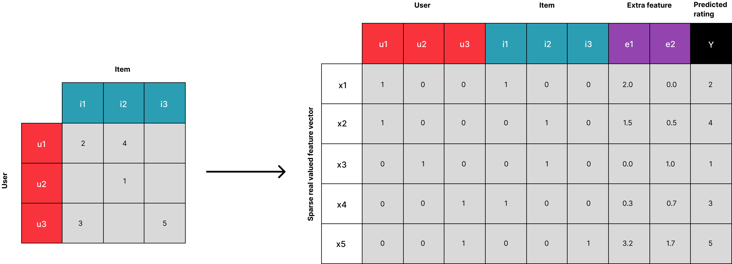
The most accessible data are explicit ratings, which include explicit input from the user regarding their level of interest in a product, i.e. the rating a user gives to an item. Usually, explicit feedback can be represented by a sparse matrix. A sparse matrix is characterized as a matrix where only a small number of fields have non-zero (or non-null) values. Since users are unlikely to rate more than a small number of items from the entirety of those available in a dataset, querying explicit information results in sparse matrices.

Of course, sparse matrices are not sufficient for training a model, and it is unreasonable to expect a complete dataset of explicit data. So, we learn the similarities a given user has with other users, and use these to predict how much they would like some unseen item.

While explicit feedback is preferable, it is also possible to use implicit feedback to reflect user behavior. Examples of implicit feedback include the browser history on a website, the number of clicks made on a given page, and a user's pattern of mouse movement. As opposed to explicit feedback, implicit feedback is represented by a densely filled matrix, because we (as researchers) can dictate how this data is to be collected or organized.

Classical recommender systems can be grouped into two main approaches: content-based (CB) and collaborative filtering (CF).

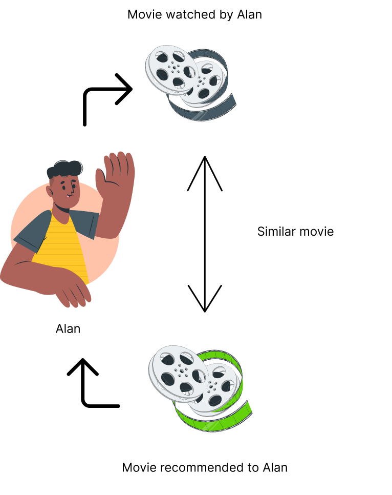
Content-based filtering generates a recommendation using additional information about the given user and item, through what we call features, which explain the observed interaction between a user and an item.

On the left is an illustration of the content-based process. If Alan has watched one movie, the recommender system will then find similar movies to it, and Alan will be given a recommendation from the set of movies most similar to the one he has already watched.

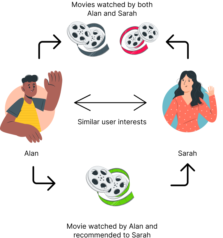
Collaborative filtering: generates a recommendation by relying on past user-item interaction, like explicit feedback (ratings) for movies watched in the past. In CF, it is sufficient to detect similar users and/or items, cluster them, and make new predictions based on the similarity existing within a cluster [6].

On the left is an illustration of the collaborative filtering process. If Alan and Sarah have watched the same movies and have the same interests, the recommender system will learn this information and recommend to Sarah a movie that Alan has watched.

The table below summarizes the advantages and disavantages of the two approaches. For more in-depth information, take a look at these references: [11, 12, 13].

	Content-based	Collaborative Filtering
Advantages	Does not require any data about the other users Can recommend items which are relevant to the user, but not the population (niche items)	Does not require domain knowledge Helps users discover new interests
Disadvantages	Requires a lot of domain knowledge Makes recommendatios based only on the existing interests of the user (no niche items)	Cannot handle fresh items or users (the Cold-Start Problem)

Matrix Factorization: a collaborative filtering method

Matrix Factorization (MF) is a class of collaborative filtering techniques [3]. In its most simplistic implementation, MF characterizes both the items and the users by a vector of factors (matrices), which then generate latent features (embeddings) when they are multiplied together (into the matrix dot product).

This method has become popular because it offers flexibility for modeling real-life scenarios, while maintaining robust scalability and predictive accuracy [2]. The toy example below includes only a very limited number of features in both the user and item matrices, allowing us to follow how predictions are computed, and understand how to interpret the effect that an individual feature may have on a given prediction. When this method scales up to a more realistic number of features, the ability to interpret the prediction is lost [19]. There exists much academic debate on uncovering the explainability of latent factor models. To learn more about it, see the following references [19, 20, 21, 22].

This box is interactive! Hover over the matrices below to learn how they are used to calculate the dot product (and make a recommendation)

User matrix

Item matrix

Rating matrix

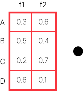
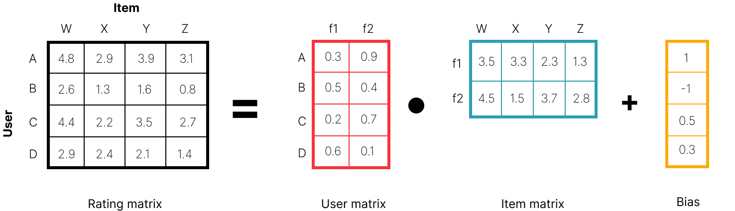
The user matrix stores the users' item-feature preferences. Here, the 4 users set 2 feature preferences in a range of [0,1].

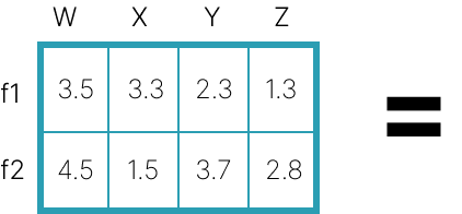
The item matrix stores the items' feature scores. Here, each of the 4 items contains 2 features.

The rating matrix stores the dot product of the user and item matrices.

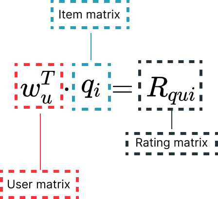
Each item i and user u are associated with a vector q_i and w_u, respectively. For a given item, the corresponding vector measures the degree to which a feature represents the item. Similarly, the user vector w_u measures the degree of interest the user has in the item.

The interaction, defined as the interest of the user u in item i , is then captured by the dot product of these two vectors. Once all the dot products are computed, it becomes possible to rank the predicted ratings and identify the best item to recommend to any given user.

Matrix Factorization formula.

This box is interactive! Adjust your preferences through the movie genre sliders for comedy and horror, and then click on Calculate Matrix Factorization to see how your preferences align with those of your friends'

Let's consider the following example: you are planning a movie night with your friends Anna, Jonny, and Kimi. You know that Anna likes both horror movies and comedy, Jonny has a strong preference for comedy, and Kimi prefers horror movies, but also enjoys comedy once in a while. To find a movie that everyone will enjoy, you are going to use a recommender system based on the Matrix Factorization techniques described above.

Comedy preference:

Horror preference:

User	Comedy	Horror
Anna	0.6	0.5
Jonny	0.7	0.1
Kimi	0.4	0.9
You	0.5	0.5

Item	Comedy	Horror
Zombieland	3	2
Modern Times	5	1
The Grudge	1	5

Calculate Matrix Factorization

How to read the results: to help you decide which movie to watch, look at the last row of the Matrix Factorization results. This row represents each movie's average predictive rating within your group.

While Matrix Factorization can produce good results in a short time, a naïve approch has a time complexity of O(mnk), where m are the number of users, n the number of items, and k the number of latent factors (a hyperparameter) [24]. This method has its disavantages:

• Cold start problem: The matrix cannot handle fresh items, such as new movies or new users the training data did not include [14].
• Recommendation relevance: Matrix Factorization uses the dot product to recommend items. If all users have interacted and liked the same item, the recommendation will focus on that item.
• Hard feature encoding: In order to generate a recommendation, we have to explicitly provide the system with user preferences and item features.

Embedding powered systems

Nowadays, recommender systems consider many more features than our MF example above:

• Categorical: userID, itemID, item brand, genre, language, etc.
• Numerical: price, delivery time, number of reviews, average of the reviews, etc.
• Unstructured: keywords, colors, material, review text, etc.

In a real-world scenario, we likely would not have explicit data on the preferences of every user and the features of every item. This hinders our ability to make optimal recommendations. How might we resolve this?

EmbeddingMF: An embedding approach to matrix factorization

Building on top of our previous approach, Matrix Factorization, we learn the latent factors (implicit characteristics) for each movie and user, based on user-movie ratings. Learning these characteristics can be done through approaches like gradient descent [16].

We will use the EmbeddingMF approach, which includes a general bias term on top of our existing dot product. EmbeddingMF is a simplification of the FunkSVD method. FunkSVD, unlike our EmbeddingMF model, incorporates at least three separate bias terms (general, user, item), on top of the matrix factorization [2].

Note: Our inclusion of a single bias term serves to broadly illustrate to the reader the effect of bias on an RS model. So, although EmbeddingMF is not the most effective or cutting-edge RS, it is sufficient for our purposes.

Augmented MF computation required for EmbeddingMF. Note the addition of the bias term (in yellow).

We start by creating two embedding matrices:

1. A user embedding matrix U, containing one user per row and n user features, as columns.
   E.g. For a set of 100 users and 200 features, U will have dimensions of (100, 200)
2. A movie embedding matrix M, containing one movie per row and n movie features, as columns.
   E.g. For a set of 100 movies and 200 features, M will have dimensions of (100, 200)

Having the same number of columns in each matrix makes the dimensions favourable for multiplying the two embedding matrices (U x M^T ). After multiplication, we add bias terms to each user and each movie. Adding bias to our matrix product results in a matrix representing predictive user ratings for all the movies in our dataset. Since these latent factors (features) are initialized randomly (independently and identically distributed Normal samples, i.i.d), the initial ratings computed by the model will likely differ significantly from the ground truth. Through training, the difference between our latent factors and the ground truth is minimized.

The model consists of a user matrix of dimensions (n_users x 128 features), a movie matrix of dimensions (n_movies x 128 features), a user bias vector of length [n_users], and a movie bias vector of length [n_movies]. We randomly initialize the latent factors for every user and movie with i.i.d samples from a Normal of mean 0 and standard deviation of 0.01. After the multiplication of users and movies, we apply a sigmoid range transformation that squeezes the results to values between 0 and 5.5. We chose to use 5.5 so that the distribution of the error for those movies whose true rating is 5 is not always negative. This allows the model to learn values only within this range for its predicted ratings. We trained the model over 15 epochs using the Mean Squared Error loss (MSELoss), a learning rate of 0.005, and a weight decay of 0.1 [17]. Since these hyperparameters gave us sufficiently robust results, we did not tune them further.

EmbeddingMF was able to generate movie rating predictions with an average validation error of 0.71. The dataset used to train and test the model included the MovieLens 1M columns of user ID, movie ID, and the movies' genres. However, MovieLens 1M also provides data on user occupations, ages, and locations (via US zip codes). How might we leverage this metadata in improving our validation error?

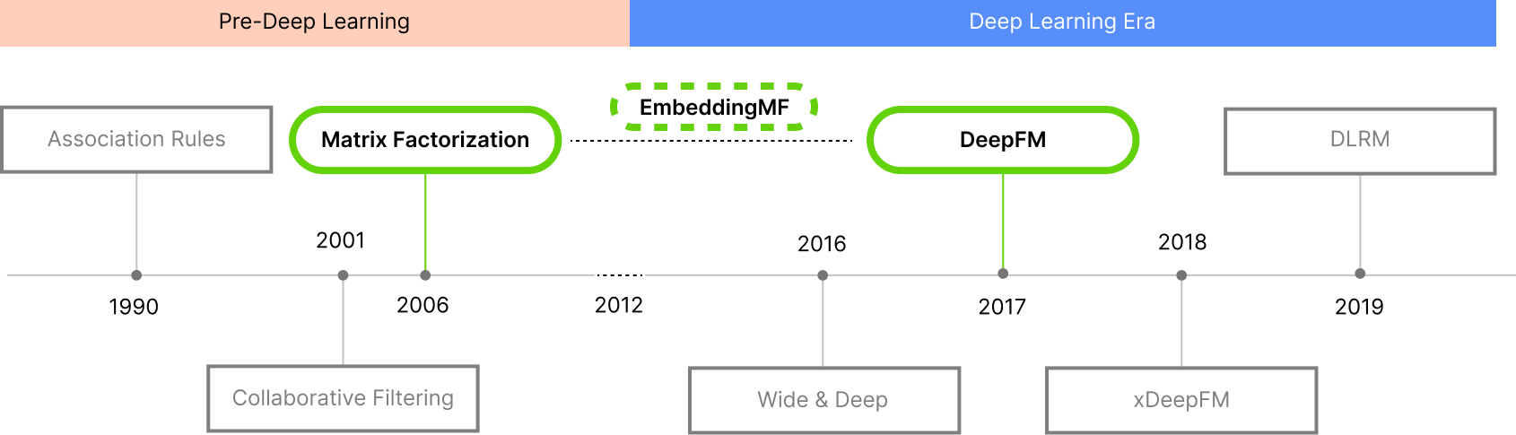
DeepFM: A deep learning factorization machine

The adoption of deep learning models has been on the rise in every domain, and recommender systems are no exception. In this section, we build upon Matrix Factorization, turning it into something we call a factorization machine (FM). More on that in a minute. The example we use to a factorization machine (FM)-based neural network. DeepFM is a deep learning recommender system developed by Guo et. al. for Huawei in 2017 [6]. The DeepFM model has a structure that considers several concepts we have discussed above, combining these into a (then considered) novel neural network architecture.

We haven't covered FMs yet-- this is coming up, don't fret!

DeepFM's output unit combines information from two components: a factorization machine, and a neural network. Both of these components accept a shared input of raw (sparse) feature data. The neural network learns dense embeddings from the sparse data, uncovering patterns pointing to both low- and high-order interactions between features. It models low-order feature interactions like FM, and models high-order feature interactions like DNN. Due to the relationships between the FM and NN, this model can learn recommendations without any additional feature engineering, and can accomodate input data which includes vectors of varying lengths. DeepFM's initial dense embedding layer compresses the input to a low-dimensional, low-sparsity, real-value vector, before further this into the FM, and the first hidden layer of the deep component. No matter how sparse our input data may be with respect to various features, DeepFM learns embeddings of the appropriate shape and appropriate sparsity for its components. We choose DeepFM for our next recommendation system progression because machine factorization combines in its computation concepts of both matrix factorization with regression. When we consider that we began with a relatively simple matrix factorization, DeepFM can be seen as an upgrade to both the two models we explored above.

Architecturally, DeepFM consists of two components that share the same input: a Factorization Machine (FM), and a deep neural network.

Factorization Machines (FM): A model class combining the advantages of Support Vector Machines with factorization models [7]. FM model all interactions between variables using factorized parameters-- user-item interactions which are represented as tuples. These tuples are vectors consisting of real-valued and numeric variables that FM treats as features, learning n-way interactions between them, n being the relevant degree of interaction for the design of some given model. The computation FM conducts includes a weight for each base feature, and an interaction term representing feature combinations [23]. Particularly useful in data contexts with high sparsity! Including the FM component as part of the overall DeepFM architecture, in addition to the DNN component, eliminates the need to pre-train the features by FM, allowing us to jointly train the combined model (FM + DNN) end-to-end. The outputs of the FM become latent feature vectors, and used as network weights in the output units of the overall model (rather than a random initialization).

On the right a represenation of Matrix Factorization which inputs are user-item interactions. On the left a Factorization Machine where the user-item interactions are represented by tuples of real-valued feature vectors and numeric target variables.

Deep component: The deep component is a feed-forward neural network, used to learn both low- and high-order feature interactions. That means that, for a given feature i, a weight w_i represents its order-1 (linear) importance, and a latent vector V_i is used to measure the impact of interactions feature i has with other features the model considers. This latent vector V_i is then fed to the FM component, to model order-2 (pairwise) feature interactions. The result, y_FM , is then fed to the deep component, to model the high-order feature interactions.

All parameters are trained jointly, rather than pre-training via the FM and then applying the DNN. The combined prediction y is represented by the following formula:

Mathematical formula to describe the output of the DeepFM model.

Our DeepFM model considers users, movies and their genres, and the users' occupation as an additional information not included in EmbeddingMF. The FM outputs a latent vector of dimensions (128,128), the same number of features as EmbeddingMF. We trained the model over 100 epochs, with a batch size of 2048, using MSELoss, and a dropout rate of 0.5 [6]. Our training of DeepFM concluded in a validation error of 0.7553, comparable to our implementation of EmbeddingMF.

One recommender cannot rule them all

All models are wrong, but some are useful.

- George Box, 1976, [15]

We have trained EmbeddingMF and the DeepFM for the task of generating recommendations with a train/test set split of 900k/100k entries of users' movie ratings [18]. By plotting the distribution of the true and predictive ratings below, we note that that the distribution of the DeepFM is very narrow and highly dense around a rating of 3.2, while that of EmbeddingFM has a density focused around 3.7. What is surprising here are the mean predictive ratings, which despite quite differing density shapes are, in fact, very close to each other— and to the training mean.

Distribution and mean of the predictive models' and training data's ratings across all movies

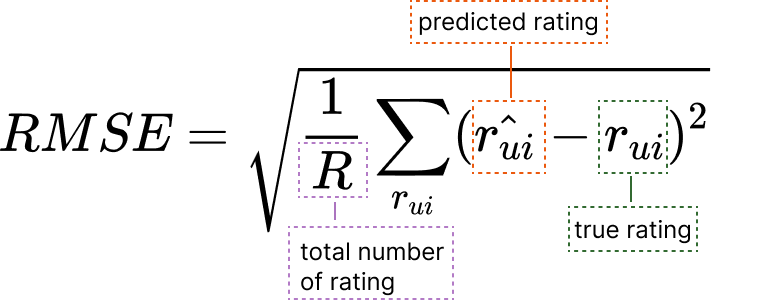
To better understand these results, we validate our models using the Root Mean Squared Error (RMSE), a standard metric widley used for validation in the recommender systems research. We decides to use RMSE over other evalutation metrics, like MAP or nDCG, for its understand semplicity. Moreover, RMSE is typically used when we want to evaluate a predicted score, such as the predictive rating of a movie, and compare it to a ground truth (true rating) as we want to do in our case. Compared to other metrics, RMSE penalizes more harshly a larger absolute error, giving you a measure of how concentrated your data is around the curve you have fit through your model. Lower RMSE translates to better recommendation accuracy [1, 8].

Root Mean Square Error formula.

By plotting the RMSE of the two models we notice that both EmbeddingMF and DeepFM present a high RMSE value at the two extremes: predicted ratings of 1 to 2 and of 5. The error on the lower rating extreme might be explained by considering that people are more willing to share positive experiences than negative ones, and so as a result we tend to train more around positive ratings than negative ones [9]. How might we explain the upper extreme?

RMSE of EmbeddingMF (yellow) and DeepFM (grey), both featuring large RMSE values at the two extremes of true ratings (x axis)

We define a perfect recommendation system as one which will recommend to users only movies they will be likely to give a rating of 5 (as a proxy for a high level of enjoyment of the recommendation). The above plot shows that both the systems we have experiemented with, while more competent than prediting the low rating of a movie, are not particularly perfect under our defined criterium. We dig deeper into this concerning finding by exploring how our two models generated movie recommendations for Xiao, as example user. Explore with us by examining the Venn diagram below.

Description of the different areas of the Venn Diagram, which examines 3 sets of movies: true ratings (movies rated 5 by the users), EmbeddingMF predicted ratings, and DeepFM predicted ratings.

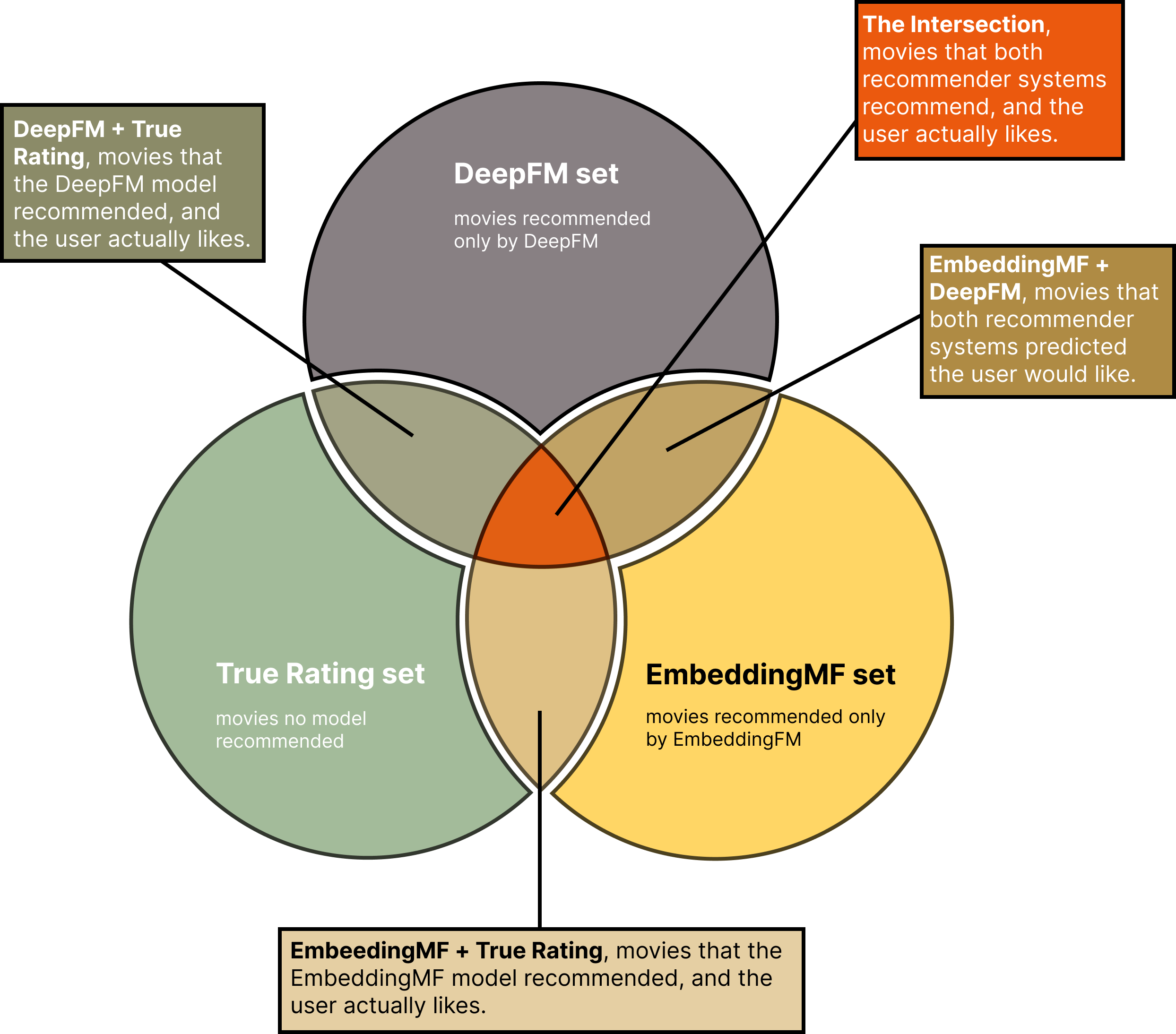
This box is interactive! The movies are represented by dots in the different sets and intersections of the Venn Diagram. The line that starts from the center of the circle represents the error (RMSE) that the model made in generating the rating prediction. Hover over one a point to discover the movie's name, its true rating, and its predicted scores from the model(s)

Let's consider Xiao. He is a young writer, between 25-34 years old, living in the West Coast (USA). We want to better understand his preferences and what the two recommenders should, and have, recommended to him. To this end, we have retrieved the top 10 movies from both the recommendation models, and a set of movies that Xiao himself has ranked 5. We examine the intersections of these sets by visualizing them in a Venn diagram, as described in our annotated legend above.

EmbeddingFM

DeepFM

The model underestimated the user's rating

The model overestimated the user's rating

Interesting to note in the above diagram are two movies with particularly large radii, located in the top left of the true rating set, and in the intersection between the two models. The former movie is one that, in truth, the user has liked and rated 5, but neither of the models decided to recommend. The latter movie is one that both models predicted that the user would like, but in truth, the user has rated 1! How did this happen?

We want to further explore these cases, where the movies recommended and the user preferences do not overlap, so that we can determine if any sort of bias might be plaguing our models.

Dashed lines in grey (DeepFM) and yellow (EmbeddingMF) reflect the prediction of each model for Xiao (User 1680)

Looking at these (true) ratings distributions, we notice a skew and an elongated tail to each histogram. In the case of Buffy, the distribution leans left and the models' mean predictions are fairly high. Despite the fact that we know Xiao hated Buffy, this suggests that, on average, users enjoyed it. Who's That Girl? shows us the opposite trend, with the added observation that the mean predicted ratings of EmbeddingMF and DeepFM deviate much less from the training set's mean rating, likely because of its substantially lower number of ratings (88 in total to Buffy's 465). What might have caused this?

Maybe some characterists of Xiao's were overlooked, making him an outlier in these rating sets? Let us see the user trends (for users' occupation, we exclude from consideration the MovieLens category 0: undefined):

Buffy the Vampire Slayer

• Reported gender breakdown: male 351, female 114
• Reported user occupations (top 3): 79 college/grad student, 36 executive/managerial, 34 technician/engineer. For writers like Xiao, we see 21 ratings
• Reported age brackets (top 3): 197 (25-34), 127 (18-24), 68 (35-44)

Who's That Girl?

• Reported gender breakdown: male 52, female 36
• Reported user occupations (top 3): 15 college/grad student, 9 executive/managerial and sales/marketing, 8 academic/educator. For writers like Xiao, we see 3 ratings
• Reported age brackets (top 3): 45 (25-34), 20 (18-24), 17 (35-44)

Conclusion

Why didn't Xiao like the movies DeepFM and EmbeddingMF recommended to him? A system is rarely aware of what it does not know, and is limited by the data it is provided for training. What if these features, this metadata, are not the correct sources of information for predicting what our user may like to watch? Xiao was so similar to the demographics of the users who enjoyed Buffy the Vampire Slayer, yet his true rating for this movie was 1. What aspects of Buffy were responsible for Xiao's dislike?

How we might learn the answer to this question, and how we might collect data for recalibrating recommender models to specific user needs, are open questions in the field of recommender systems research. While recommender systems aim to generate a personalized experience on the web, models are trained on a group of users with similar characteristics, not on a single user and their individual opinions. Through exploration of Xiao's top recommendations, we have seen that the features we have used for characterizing user similarities may not be sufficient for making good recommendations. Such exploration has allowed us insight, beyond model fit and validation losses, into the fact that there are some features out there, missing from our models, that can make our recommendations into the personalized experience we seek.

What do we ask users to learn these niche recommendations? How do we collect, or compute, such abstract data representations? The discovery of machine-recommended content that speaks to, and connects with us on a personal level may require moving beyond a one-model-fits-all-users approach. Calibrating our models per-user, through specific user feedback and desires, could be the key to reaching our personalized recommendation dreams— and finally answering that one infuriating question:

What should we watch tonight?

References

References

1. Science and statistics  Journal of the American Statistical Association, vol. 71, no. 356, 1976, pp. 791-99
   Box, George EP, 1976.

[1] Ricci, Francesco, Lior Rokach, and Bracha Shapira. "Introduction to recommender systems handbook." Recommender systems handbook. Springer, Boston, MA, 2011. 1-35.

[2] Koren, Yehuda, Robert Bell, and Chris Volinsky. "Matrix factorization techniques for recommender systems." Computer 42.8 (2009): 30-37.

[3] Lee, Daniel D., and H. Sebastian Seung. "Learning the parts of objects by non-negative matrix factorization." Nature 401.6755 (1999): 788-791.

[4] Glauber, Rafael, and Angelo Loula. "Collaborative filtering vs. content-based filtering: differences and similarities." arXiv preprint arXiv:1912.08932 (2019).

[5] Cheng, Heng-Tze, et al. "Wide & deep learning for recommender systems." Proceedings of the 1st workshop on deep learning for recommender systems. 2016.

[6] Guo, Huifeng, et al. "DeepFM: a factorization-machine based neural network for CTR prediction." arXiv preprint arXiv:1703.04247 (2017).

[7] Rendle, Steffen. "Factorization machines." 2010 IEEE International conference on data mining. IEEE, 2010.

[8] Isinkaye, Folasade Olubusola, Yetunde O. Folajimi, and Bolande Adefowoke Ojokoh. "Recommendation systems: Principles, methods and evaluation." Egyptian informatics journal 16.3 (2015): 261-273.

[9] 2018 Customer Experience, https://www.sitel.com/report/2018-cx-index/

[10] Deisenroth, Marc Peter, A. Aldo Faisal, and Cheng Soon Ong. Mathematics for machine learning. Cambridge University Press, 2020.

[11] Pazzani, Michael J., and Daniel Billsus. "Content-based recommendation systems." The adaptive web. Springer, Berlin, Heidelberg, 2007. 325-341.

[12] Sharma, Ritu, Dinesh Gopalani, and Yogesh Meena. "Collaborative filtering-based recommender system: Approaches and research challenges." 2017 3rd international conference on computational intelligence & communication technology (CICT). IEEE, 2017.

[13] Hannon, John, Mike Bennett, and Barry Smyth. "Recommending twitter users to follow using content and collaborative filtering approaches." Proceedings of the fourth ACM conference on Recommender systems. 2010.

[14] Lika, Blerina, Kostas Kolomvatsos, and Stathes Hadjiefthymiades. "Facing the cold start problem in recommender systems." Expert systems with applications 41.4 (2014): 2065-2073.

[15] Box, George E. P. (1976), "Science and statistics" (PDF), Journal of the American Statistical Association, 71 (356): 791-799, doi:10.1080/01621459.1976.10480949.

[16] Ruder, Sebastian. "An overview of gradient descent optimization algorithms." arXiv preprint arXiv:1609.04747 (2016).

[17] https://towardsdatascience.com/various-implementations-of-collaborative-filtering-100385c6dfe0

[18] F. Maxwell Harper and Joseph A. Konstan. 2015. The MovieLens Datasets: History and Context. ACM Transactions on Interactive Intelligent Systems (TiiS) 5, 4: 19:1–19:19. https://doi.org/10.1145/2827872

[19] Zhang, Yongfeng, et al. "Explicit factor models for explainable recommendation based on phrase-level sentiment analysis." Proceedings of the 37th international ACM SIGIR conference on Research & development in information retrieval. 2014.

[20] Abdollahi, Behnoush, and Olfa Nasraoui. "Using explainability for constrained matrix factorization." Proceedings of the eleventh ACM conference on recommender systems. 2017.

[21] Alhejaili, Abdullah, and Shaheen Fatima. "Expressive Latent Feature Modelling for Explainable Matrix Factorisation based Recommender Systems." ACM Transactions on Interactive Intelligent Systems (TiiS) (2022).

[22] Abdollahi, Behnoush, and Olfa Nasraoui. "Explainable matrix factorization for collaborative filtering." Proceedings of the 25th International Conference Companion on World Wide Web. 2016.

[23] Lundquist, Eric. “Factorization Machines for Item Recommendation With Implicit Feedback Data.” Medium, 30 Mar. 2022, towardsdatascience.com/factorization-machines-for-item-recommendation-with-implicit-feedback-data-5655a7c749db.

[24] Arora, Sanjeev, et al. "Computing a nonnegative matrix factorization--provably." Proceedings of the forty-fourth annual ACM symposium on Theory of computing. 2012.

Reuse

Diagrams and text are licensed under Creative Commons Attribution CC-BY 4.0 with the source available on GitHub, unless noted otherwise. The figures that have been reused from other sources don’t fall under this license and can be recognized by a note in their caption: “Figure from …”.